Goddard Rocket Landing

Edit me

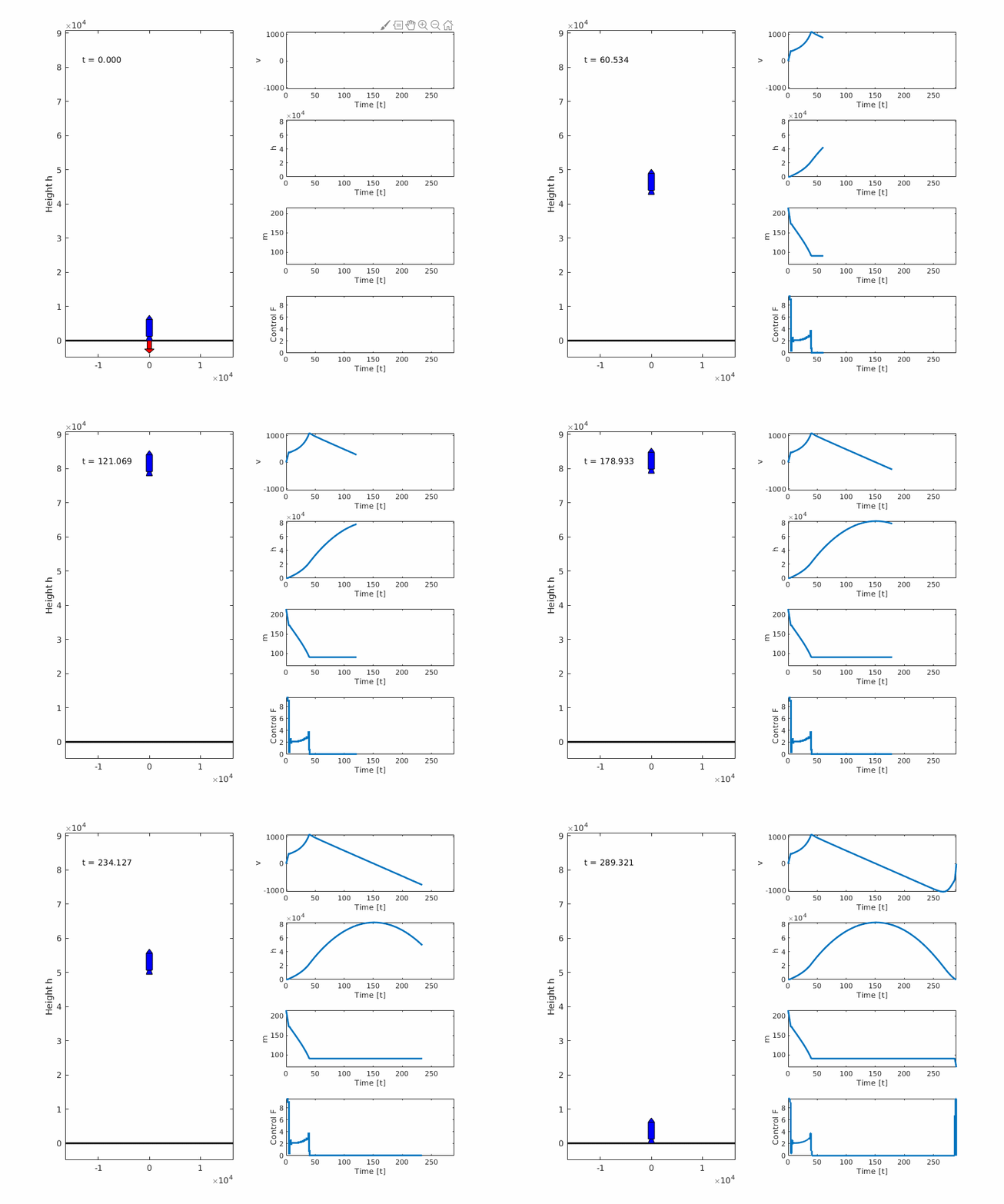
This is the same model as in the Goddard rocket free final time and Goddard rocket fixed final time examples but this time the rocket has maximize the altitude and still have enough fuel left to land softly.

goddardRocketFreeTfAnimation — Goddard rocket landing animation

Problem formulation

The problem formulation is the following:

$\max \: h(t)$ $\dot{v} = \frac{F \cdot c - \textrm{sign}(v) D(h,v)}{m}-g(h)$ $\dot{h} = v$ $\dot{m} = - F$ $D(h,v) = D_0 v^2 exp( -\beta h )$ $g(h) = g_0\Big(\frac{r0}{r0+h} \Big)^2$ $m(0) = 214.839$ $v(0) = 0$ $h(0) = 0$ $m(t_f) = 67.9833$ $v(t_f) = 0$ $h(t_f) = 0$ $g_0 = 9.81$ $r_0 = 6.371e6$ $0 \leq F \leq 9.525515$ $D_0 = 0.01227$ $c = 2060$ $\beta = 0.145e-3$

The states are the rocket velocity $v$ , the altitude from the ground $h$ and mass of the rocket $m$ . The rocket burns fuel and expels it out the nozzle creating thrust, in the model the fuel flow rate $F$ is the control and the ratio between thrust and change in mass is $T = F \cdot c$ .

Yop implementation

This example show how to solve a problem with two phases. It also shows how to take out the air resistance force out of the model and then plot it in a 3d graph.

%% Goddard Rocket Landing
% Author: Dennis Edblom
% Create the Yop system
sys = YopSystem('states', 3, 'controls', 1, ...
    'model', @goddardRocketModel1);
time = sys.t;
% Rocket signals (symbolic)
rocket = sys.y.rocket;

%% Formulate optimal control problem
ocp(1) = YopOcp();
ocp(2) = YopOcp();

% Constants
m0 = 214.839;
mf = 67.9833;
Fm = 9.525515;

% Phase 1
ocp(1).max({ t_f( rocket.height ) });
ocp(1).st(...
     'systems', sys, ...
    ... % initial conditions
    { 0   '==' t_0(time)            }, ...
    { 0   '==' t_0(rocket.velocity) }, ...
    { 0   '==' t_0(rocket.height)   }, ...
    { m0  '==' t_0(rocket.mass)     }, ...
    ... % Constraints
    {  0  '<=' rocket.height       '<=' inf }, ...
    { mf  '<=' rocket.mass         '<=' m0  }, ...
    {  0  '<=' rocket.fuelMassFlow '<=' Fm  } ...
    );

% Phase 2
ocp(2).min({ t_f( 0 ) });
ocp(2).st(...
     'systems', sys, ...
    ... % Initial conditions
    {  0  '<=' t_0(time) '<=' inf }, ...
    ... % Constraints
    {  0  '<=' rocket.height       '<=' inf }, ...
    { mf  '<=' rocket.mass         '<=' m0  }, ...
    {  0  '<=' rocket.fuelMassFlow '<=' Fm  }, ...
    ... % Final conditions, for landing
    {  0  '==' t_f(rocket.velocity) }, ...
    {  0  '==' t_f(rocket.height)   } ...
    );

% Scaling the objective
ocp(1).scale('objective', 1e-4);
ocp(2).scale('objective', 1e-4);

% Solving the OCP
sol = ocp.solve(...
    'controlIntervals', 100, ...
    'polynomialDegree', 3, ...
    'collocationPoints', 'radau' ...
    );

%% Plot the results
figure(1)
subplot(311); hold on
sol(1).plot(time, rocket.velocity)
sol(2).plot(time, rocket.velocity)
xlabel('Time')
ylabel('Velocity')

subplot(312); hold on
sol(1).plot(time, rocket.height)
sol(2).plot(time, rocket.height)
xlabel('Time')
ylabel('Height')

subplot(313); hold on
sol(1).plot(time, rocket.mass)
sol(2).plot(time, rocket.mass)
xlabel('Time')
ylabel('Mass')

figure(2); hold on
sol(1).stairs(time, rocket.fuelMassFlow)
sol(2).stairs(time, rocket.fuelMassFlow)
xlabel('Time')
ylabel('F (Control)')

figure(3); hold on
sol(1).plot3(rocket.height , rocket.velocity, sys.y.drag.force, 'LineWidth',2)
sol(2).plot3(rocket.height , rocket.velocity, sys.y.drag.force, 'LineWidth',2)
xlabel('h')
ylabel('v')
zlabel('Fa')
grid minor

%% Model
function [dx, y] = goddardRocketModel1(t, x, u)
% States and control
v = x(1);
h = x(2);
m = x(3);
F = u;

% Parameters
D0   = 0.01227;
beta = 0.145e-3;
c    = 2060;
g0   = 9.81;
r0   = 6.371e6;

% Drag and gravity
D   = D0*exp(-beta*h);
F_D = sign(v)*D*v^2;
g   = g0*(r0/(r0+h))^2;

% Dynamics
dv = (F*c-F_D)/m-g;
dh = v;
dm = -F;
dx = [dv;dh;dm];

% Signals y
y.rocket.velocity     = v;
y.rocket.height       = h;
y.rocket.mass         = m;
y.rocket.fuelMassFlow = F;
y.drag.coefficient    = D;
y.drag.force          = F_D;
y.gravity             = g;
end

Plots

goddardLandingStates — Goddard rocket landing states

goddardLandingControl — Goddard rocket landing control

goddardLanding3d — Goddard rocket 3d plot of drag, velocity and height